Matching using real images

In this experiment we perform the matching between two omnidirectional images acquired with an hypercatadioptric system. We compute the scale space using our approach, then this scale-space is passed to Vedaldi's software to compute the extrema points and the descriptors.

Extrema points features detected with LB



Normal SIFT points



Matching of LB features



Matching of SIFT features

The difference is explained since the scale-spaces used by the two approaches are different. The LB approach has smoothed images in the first two octaves but less smoothed in the las two. The opposite happens with Vedaldi's application, the first two octaves are less smtoothed and the last two are more smoothed than the LB ones.

Scale Space computed with LB

Normal SIFT Scale Space

Matching Experiments using Shape Context Locally

In this experiment we extract the edges of the images using Canny algorithm. For each extracted point we compute its corresponding support region based on the scale where the feature was detected. With all the edge pixels contained in this area we compute the histogram corresponding to that particular point. The approach used is taken from [1], with a log-polar grid of five ringsf and twelve sectors. The histogram-desciptor is a n x 60 matrix, where n is the number of edge points contained in the support region. The match process is performed using [2].

Edges with extrema points and descriptor example

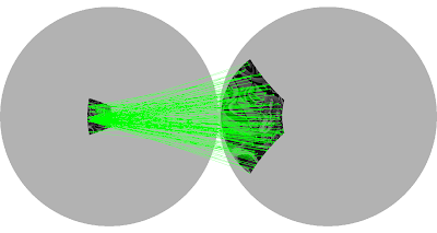
Matching Results

We observe that some points have several matches which is not correct. This is possible caused by either the similarity matrix required by [2] or by the descriptor.

In the next experiment we change the descriptor. In this case the descriptor is only the 1x60 histogram counting the number of edge pixels in each cell. The results are similar to the previous case. We need to explore more the distance between the histograms we are using.

[1] G. Mori, S. Belongie, and J. Malik. "Shape Contexts Enable Efficient Retrieval of Similar Shapes".CVPR 2001
[2] Ofir Pele and Michael Werman. "The Quadratic-Chi Histogram Distance Family". ECCV 2010.

Matching Experiments using SIFT descriptors

In this experiments we use Vedaldi's software. We provide the scale space and the software computes the points and descriptors. Then using the same sotware we match the points.

Matching using LB scale space

Matching using SIFT

We observe that the SIFT implementation performs better that the one using the LB approach. This is because the scale space we computed has different scales from the ones that are used by the implementation. Even we change the number of octaves and scales, internally the initial scale is not changed. The descriptors use this scale and it might be the reason the are badly computed.

Matching Experiments using NCC

The detected features in the 1s image (rotated 40degrees in z-axis) are located in the second image (-10 degrees in z-axis) using NCC. The size of the template is determined by the scale where the feature was detected.

We observe that the matching does not perform well, since the scale where the feature was detected in the image plane is not representative of the real size of the patch we are looking for in the second image.

Matching Experiments using Shape Context

We perform experiments matching the SIFT points and the extrema points extracted using our LB algorithm. We use the shape context approach proposed by Belongie et al.[1] and the software available at his website to compute the descriptors based on the extracted points. The matching algorithm uses the approach proposed by Ofir Pele and Michael Werman [2]. The code is available at the author's webpage.

Matching LB points

The first experiment matches the 2 point sets obtained using our approach:

We observe that the points in the second image are mostly located on the periphery.

Matching SIFT points

Since the shape context approach considers the points as a unity, i.e., the points are related to each other in a certain way. That structure should be preserved from one image to the other.

The following example uses the extracted points using our approach in the first image and the SIFT points in the second. Coincidently the structure of the set points are similar.

Matching LB points with SIFT points

We need to explore this situation and to evaluate if the shape context approach with the extracted points seen as sets of points are suitable for the matching step.

[1] G. Mori, S. Belongie, and J. Malik. "Shape Contexts Enable Efficient Retrieval of Similar Shapes".CVPR 2001

[2] Ofir Pele and Michael Werman. "The Quadratic-Chi Histogram Distance Family". ECCV 2010.

Repeatability Experiment

We perform rotations from -40 degrees to 40 degrees in x-axis and y-axis. The transformations of the image corresponding to the y-axis are more drastic. We show the images corresponding to -40 degrees and 40 degrees rotations in both axes.

Y-AXIS

X-AXIS

We show the feature obtained with the LB approach in the rotations around the y-axis (-40º and 40º)

Now we show the results of the repeatability experiment, compared to the normal Scale Space obtained by SIFT (we use Vedaldi's implementation to modify the number of scales and octaves).

Computing the Scale Space using the Laplace-Beltrami Operator (LPO)

Using the LBO we compute the scale space of omnidirectional images. We use the initial scale scale_0 = 0.8 and the definition of Arican's t_i = k^(2i)*scale_0^2. In opposition to other approaches that use the standard deviation. The full set of scales used are:

scale 1 = 0.8

scale 2 = 1.0159

scale 3 = 1.61.27

scale 4 = 2.56

We use the last image in each scale downsampled as the first one in the next scale. Here we show the first and last octaves.

FIRST OCTAVE

LAST OCTAVE

When the scale space is built, we perform the steps of the normal SIFT. We compute the differences of smoothed images to approximate the Laplacian of Gaussians (LoG). We observe the differences correspondig to the first and last octaves.

FIRST OCTAVE

LAST OCTAVE

Then the extrema are computed. Here we observe some results for different rotations and scales.

ORIGINAL AND DOUBLE SCALED:

ORIGINAL AND ROTATED